Process and plot JEDI diag (jdiag) results#
JEDI or GSI generates observation space diagnostic files, which contains original observation information, hofx (H(x), i.e. model counter-parts at the observataion locations), OMB (observation minus background), OMA as well as other information.
This notebook covers how to deal with JEDI diganostic files (which are also called output ioda files). We call them jdiag files.
import packages and define variables#
%%time

# autoload external python modules if they changed
%load_ext autoreload
%autoreload 2

import os, sys
pyDAmonitor_ROOT=os.getenv("pyDAmonitor_ROOT")
if pyDAmonitor_ROOT is None:
    print("!!! pyDAmonitor_ROOT is NOT set. Run `source ush/load_pyDAmonitor.sh`")
else:
    print(f"pyDAmonitor_ROOT={pyDAmonitor_ROOT}\n")
sys.path.insert(0, pyDAmonitor_ROOT)

# import modules
import warnings
import math
import numpy as np
import uxarray as ux
import xarray as xr
import pandas as pd
import seaborn as sns  # seaborn handles NaN values automatically
import matplotlib.pyplot as plt
from netCDF4 import Dataset
from DAmonitor.base import query_dataset, query_data, query_obj, to_dataframe, aircraft_reject_list_to_df

#jdiag_file=f"{pyDAmonitor_ROOT}/data/ioda/ioda_aircar.2024050600.nc"
jdiag_file=f"{pyDAmonitor_ROOT}/data/mpasjedi/jdiag_aircar_t133.nc"
pyDAmonitor_ROOT=/gpfs/f6/arfs-gsl/world-shared/gge/tmp/pyDAmonitor
CPU times: user 24.7 s, sys: 637 ms, total: 25.4 s
Wall time: 4.1 s
Use the obsSpace class to read jdiag files#
from DAmonitor.obs import obsSpace, fit_rate
# create a t133 object using the obsSpace class
t133=obsSpace(jdiag_file)
# check the t133 object
query_obj(t133)
['ds',
 'filepath',
 'groups',
 'locations',
 'metadata',
 'nlocs',
 'q',
 'rh',
 't',
 'td',
 'u',
 'v']
np.set_printoptions(threshold=np.inf)  # print out all array values
# print(t133.t.aircraftFlightNumber)
# print(t133.t.stationIdentification)
print(t133.t.stationIdentification[10])
print(t133.t.aircraftFlightNumber[10])
#
np.set_printoptions(threshold=500) # don't print out all array values
print(t133.t.ObsValue)
VTTDSIZA
C4GBTSZA
[279.25 273.55 279.25 ... 282.05 292.75 304.25]
# query data
query_data(t133.q)  # since the t133 object does not contain q observations, so it will display meta information
stationIdentification, aircraftFlightPhase, timeOffset, prepbufrDataLvlCat, longitude, stationElevation, latitude, prepbufrReportType, pressure, dateTime, height, dumpReportType, aircraftFlightNumber, ObsError, ObsType, ObsValue, QualityMarker, Location
# query data
query_data(t133.t)
EffectiveError0, EffectiveError1, EffectiveError2, EffectiveQC0, EffectiveQC1, EffectiveQC2, stationIdentification, aircraftFlightPhase, timeOffset, prepbufrDataLvlCat, longitude, stationElevation, latitude, prepbufrReportType, pressure, dateTime, height, dumpReportType, aircraftFlightNumber, ObsBias0, ObsBias1, ObsBias2, ObsError, ObsType, ObsValue, QualityMarker, TempObsErrorData, hofx0, hofx1, hofx2, innov1, oman, ombg, Location
The above output shows that we reorganize the data structure based on the observation variable, i.e. t, q, uv, bt
We can access values easily using popular Python class strucutre, i.e. t133.t, t133.t.ObsValue, etc
Convert to Pandas DataFrame#
Converting jdiag data into Pandas DataFrame brings up lots of benefits and we can use utilize lots of mature DataFrames capabilities.
We can see this from the following cell.
pd.set_option('display.max_columns', None)  # show all dataframe columns
df = to_dataframe(t133.t)
df[df["QualityMarker"]>=0]  # filter the data frame
#df
| EffectiveError0 | EffectiveError1 | EffectiveError2 | EffectiveQC0 | EffectiveQC1 | EffectiveQC2 | stationIdentification | aircraftFlightPhase | timeOffset | prepbufrDataLvlCat | longitude | stationElevation | latitude | prepbufrReportType | pressure | dateTime | height | dumpReportType | aircraftFlightNumber | ObsBias0 | ObsBias1 | ObsBias2 | ObsError | ObsType | ObsValue | QualityMarker | TempObsErrorData | hofx0 | hofx1 | hofx2 | innov1 | oman | ombg | Location | |
|---|---|---|---|---|---|---|---|---|---|---|---|---|---|---|---|---|---|---|---|---|---|---|---|---|---|---|---|---|---|---|---|---|---|---|
| 0 | 0.821017 | 0.821017 | 0.821017 | 0 | 0 | 0 | GY0VJTBA | 5 | -3597.011963 | 6 | 247.897995 | 3139 | 40.830002 | 133 | 68880.000000 | 1782860403 | 3139 | 41 | ISQBOZRA | 0.0 | 0.0 | 0.0 | NaN | 133 | 279.250000 | 1 | 0.821017 | 279.208008 | 279.330261 | 279.354889 | -0.080262 | -0.104878 | 0.041996 | 0 |
| 1 | 0.770832 | 0.770832 | 0.770832 | 0 | 0 | 0 | FXSVFQZA | 6 | -2520.000000 | 6 | 255.546997 | 4393 | 39.834999 | 133 | 58550.000000 | 1782861480 | 4393 | 41 | 0BIDSQRA | 0.0 | 0.0 | 0.0 | NaN | 133 | 273.549988 | 1 | 0.770832 | 274.123016 | 273.747955 | 273.740021 | -0.197955 | -0.190047 | -0.573033 | 8555 |
| 2 | 0.788386 | 0.788386 | 0.788386 | 0 | 0 | 0 | FXSVFQZA | 6 | -2459.988037 | 6 | 255.498001 | 3812 | 39.785000 | 133 | 63159.996094 | 1782861541 | 3812 | 41 | 0BIDSQRA | 0.0 | 0.0 | 0.0 | NaN | 133 | 279.250000 | 1 | 0.788386 | 280.079224 | 279.770416 | 279.765747 | -0.520424 | -0.515746 | -0.829226 | 8557 |
| 3 | 0.809003 | 0.809003 | 0.809003 | 0 | 0 | 0 | FXSVFQZA | 6 | -2400.012207 | 6 | 255.507996 | 3352 | 39.720001 | 133 | 67030.000000 | 1782861600 | 3352 | 41 | 0BIDSQRA | 0.0 | 0.0 | 0.0 | NaN | 133 | 285.049988 | 1 | 0.809003 | 284.621979 | 284.948578 | 284.943298 | 0.101406 | 0.106701 | 0.428004 | 8559 |
| 4 | 0.829013 | 0.829013 | 0.829013 | 0 | 0 | 0 | FXSVFQZA | 6 | -2340.000000 | 6 | 255.511993 | 3003 | 39.657001 | 133 | 70080.000000 | 1782861660 | 3003 | 41 | 0BIDSQRA | 0.0 | 0.0 | 0.0 | NaN | 133 | 288.250000 | 1 | 0.829013 | 288.532898 | 288.535919 | 288.520844 | -0.285913 | -0.270836 | -0.282884 | 8561 |
| ... | ... | ... | ... | ... | ... | ... | ... | ... | ... | ... | ... | ... | ... | ... | ... | ... | ... | ... | ... | ... | ... | ... | ... | ... | ... | ... | ... | ... | ... | ... | ... | ... | ... | ... |
| 27727 | 0.754601 | 0.754601 | 0.754601 | 0 | 0 | 0 | QZKWUWBA | 5 | -780.012024 | 6 | 278.217010 | 8169 | 24.850000 | 133 | 34740.000000 | 1782863220 | 8169 | 41 | EPGCFGRA | 0.0 | 0.0 | 0.0 | NaN | 133 | 249.849991 | 1 | 0.754601 | 249.246582 | 249.489044 | 249.514404 | 0.360944 | 0.335580 | 0.603405 | 23415 |
| 27728 | 0.725757 | 0.725757 | 0.725757 | 0 | 0 | 0 | QZKWUWBA | 5 | -600.011963 | 6 | 278.416992 | 6370 | 25.150000 | 133 | 44840.000000 | 1782863400 | 6370 | 41 | EPGCFGRA | 0.0 | 0.0 | 0.0 | NaN | 133 | 261.149994 | 1 | 0.725757 | 261.250702 | 260.774231 | 260.810150 | 0.375756 | 0.339835 | -0.100701 | 26243 |
| 27729 | 0.827965 | 0.827965 | 0.827965 | 0 | 0 | 0 | QZKWUWBA | 5 | -299.988007 | 6 | 278.967010 | 3018 | 25.299999 | 133 | 69950.000000 | 1782863701 | 3018 | 41 | EPGCFGRA | 0.0 | 0.0 | 0.0 | NaN | 133 | 282.049988 | 1 | 0.827965 | 280.991302 | 281.227814 | 281.262054 | 0.822185 | 0.787937 | 1.058697 | 30767 |
| 27730 | 1.020571 | 1.020571 | 1.020571 | 0 | 0 | 0 | QZKWUWBA | 5 | 240.012009 | 6 | 279.382996 | 1189 | 25.716999 | 133 | 87830.000000 | 1782864240 | 1189 | 41 | EPGCFGRA | 0.0 | 0.0 | 0.0 | NaN | 133 | 292.750000 | 1 | 1.020571 | 292.154907 | 292.142029 | 292.171997 | 0.607969 | 0.578000 | 0.595104 | 37440 |
| 27731 | 7.202972 | 7.202972 | 7.202972 | 0 | 0 | 0 | QZKWUWBA | 6 | 600.011963 | 6 | 279.704987 | -21 | 25.802000 | 133 | 101580.000000 | 1782864600 | -21 | 41 | EPGCFGRA | 0.0 | 0.0 | 0.0 | NaN | 133 | 304.250000 | 1 | 7.202972 | 303.406586 | 303.599457 | 303.622955 | 0.650531 | 0.627059 | 0.843404 | 41184 |
27732 rows × 34 columns
Read the aircraft reject list from “current_bad_aircraft.txt”#
filepath=f"{pyDAmonitor_ROOT}/data/current_bad_aircraft.txt"
dflist = aircraft_reject_list_to_df(filepath)
dflist
| tailID | flagT | flagW | flagR | FSL | MDCRS | N | bs_T | std_T | bs_S | std_S | bs_D | std_D | bs_W | std_W | bs_RH | std_RH | fail_reason | |
|---|---|---|---|---|---|---|---|---|---|---|---|---|---|---|---|---|---|---|
| 0 | 00000320 | T | W | - | 26490 | -------- | 470 | 11.3 | 2.8 | 0.8 | 2.7 | -8 | 11 | 1.9 | 4.0 | 0.0 | 0.0 | Unknown(bias_Tstd_Tbias_DIR) |
| 1 | 00000400 | T | W | R | 0 | -------- | 0 | 0.0 | 0.0 | 0.0 | 0.0 | 0 | 0 | 0.0 | 0.0 | 0.0 | 0.0 | UND_Piper(resrch_T_W_R) |
| 2 | 00000450 | T | W | R | 9086 | -------- | 0 | 0.0 | 0.0 | 0.0 | 0.0 | 0 | 0 | 0.0 | 0.0 | 0.0 | 0.0 | UND_Piper(resrch_T_W_Rresrch_T_W_R) |
| 3 | 00000451 | T | W | R | 9148 | -------- | 0 | 0.0 | 0.0 | 0.0 | 0.0 | 0 | 0 | 0.0 | 0.0 | 0.0 | 0.0 | King_Air(resrch_T_W_RU_Wyo_T_W_R) |
| 4 | 00000499 | T | W | R | 0 | -------- | 0 | 0.0 | 0.0 | 0.0 | 0.0 | 0 | 0 | 0.0 | 0.0 | 0.0 | 0.0 | Unknown(TAM_FS_T_W_R) |
| ... | ... | ... | ... | ... | ... | ... | ... | ... | ... | ... | ... | ... | ... | ... | ... | ... | ... | ... |
| 278 | N988DL | - | W | - | 250 | C5M13RZA | 0 | 0.0 | 0.0 | 0.0 | 0.0 | 0 | 0 | 0.0 | 0.0 | 0.0 | 0.0 | MD88(md88_W) |
| 279 | N989DL | - | W | - | 251 | ENXL3TBA | 0 | 0.0 | 0.0 | 0.0 | 0.0 | 0 | 0 | 0.0 | 0.0 | 0.0 | 0.0 | MD88(md88_W) |
| 280 | N990AK | T | - | - | 31354 | VM3LX3RA | 924 | -0.4 | 15.6 | 0.3 | 2.1 | -1 | 7 | 1.6 | 3.0 | 0.0 | 0.0 | Unknown(std_T) |
| 281 | OE-LPL | - | W | - | 32404 | UAV15PJA | 310 | 0.9 | 0.9 | 1.1 | 2.2 | 18 | 63 | 18.1 | 21.8 | 0.0 | 0.0 | Unknown(bias_DIRstd_DIRstd_Wrms_W) |
| 282 | OE-LPM | - | W | - | 32579 | BGWUR1ZA | 269 | 0.2 | 1.0 | 1.0 | 2.3 | 11 | 65 | 17.5 | 21.0 | 0.0 | 0.0 | Unknown(bias_DIRstd_DIRstd_Wrms_W) |
283 rows × 18 columns
check if any tailID is in the jdiag stationIdentification field#
# all 283 tailIDs are NOT found in jdiag `stationIdentification` fields
mask = dflist["tailID"].isin(df["stationIdentification"])
print(len(dflist[mask]))
0
# this confirms all 283 rows are NOT found in jdiag `stationIdentification` fields
mask = ~dflist["tailID"].isin(df["stationIdentification"])
dflist[mask]
| tailID | flagT | flagW | flagR | FSL | MDCRS | N | bs_T | std_T | bs_S | std_S | bs_D | std_D | bs_W | std_W | bs_RH | std_RH | fail_reason | |
|---|---|---|---|---|---|---|---|---|---|---|---|---|---|---|---|---|---|---|
| 0 | 00000320 | T | W | - | 26490 | -------- | 470 | 11.3 | 2.8 | 0.8 | 2.7 | -8 | 11 | 1.9 | 4.0 | 0.0 | 0.0 | Unknown(bias_Tstd_Tbias_DIR) |
| 1 | 00000400 | T | W | R | 0 | -------- | 0 | 0.0 | 0.0 | 0.0 | 0.0 | 0 | 0 | 0.0 | 0.0 | 0.0 | 0.0 | UND_Piper(resrch_T_W_R) |
| 2 | 00000450 | T | W | R | 9086 | -------- | 0 | 0.0 | 0.0 | 0.0 | 0.0 | 0 | 0 | 0.0 | 0.0 | 0.0 | 0.0 | UND_Piper(resrch_T_W_Rresrch_T_W_R) |
| 3 | 00000451 | T | W | R | 9148 | -------- | 0 | 0.0 | 0.0 | 0.0 | 0.0 | 0 | 0 | 0.0 | 0.0 | 0.0 | 0.0 | King_Air(resrch_T_W_RU_Wyo_T_W_R) |
| 4 | 00000499 | T | W | R | 0 | -------- | 0 | 0.0 | 0.0 | 0.0 | 0.0 | 0 | 0 | 0.0 | 0.0 | 0.0 | 0.0 | Unknown(TAM_FS_T_W_R) |
| ... | ... | ... | ... | ... | ... | ... | ... | ... | ... | ... | ... | ... | ... | ... | ... | ... | ... | ... |
| 278 | N988DL | - | W | - | 250 | C5M13RZA | 0 | 0.0 | 0.0 | 0.0 | 0.0 | 0 | 0 | 0.0 | 0.0 | 0.0 | 0.0 | MD88(md88_W) |
| 279 | N989DL | - | W | - | 251 | ENXL3TBA | 0 | 0.0 | 0.0 | 0.0 | 0.0 | 0 | 0 | 0.0 | 0.0 | 0.0 | 0.0 | MD88(md88_W) |
| 280 | N990AK | T | - | - | 31354 | VM3LX3RA | 924 | -0.4 | 15.6 | 0.3 | 2.1 | -1 | 7 | 1.6 | 3.0 | 0.0 | 0.0 | Unknown(std_T) |
| 281 | OE-LPL | - | W | - | 32404 | UAV15PJA | 310 | 0.9 | 0.9 | 1.1 | 2.2 | 18 | 63 | 18.1 | 21.8 | 0.0 | 0.0 | Unknown(bias_DIRstd_DIRstd_Wrms_W) |
| 282 | OE-LPM | - | W | - | 32579 | BGWUR1ZA | 269 | 0.2 | 1.0 | 1.0 | 2.3 | 11 | 65 | 17.5 | 21.0 | 0.0 | 0.0 | Unknown(bias_DIRstd_DIRstd_Wrms_W) |
283 rows × 18 columns
check if any MDCRS is in the jdiag stationIdentification fields#
mask = dflist["MDCRS"].isin(df["stationIdentification"])
print(len(dflist[mask]))
dflist[mask]
34
| tailID | flagT | flagW | flagR | FSL | MDCRS | N | bs_T | std_T | bs_S | std_S | bs_D | std_D | bs_W | std_W | bs_RH | std_RH | fail_reason | |
|---|---|---|---|---|---|---|---|---|---|---|---|---|---|---|---|---|---|---|
| 29 | N12006 | - | W | - | 24180 | GN0RPDJA | 334 | 0.9 | 0.9 | 0.5 | 2.3 | 8 | 37 | 13.2 | 14.6 | 0.0 | 0.0 | Unknown(bias_DIRstd_DIRstd_Wrms_W) |
| 31 | N12012 | - | W | - | 26076 | LO5SVXJA | 401 | 0.8 | 1.0 | 0.6 | 2.2 | 6 | 59 | 19.5 | 22.4 | 0.0 | 0.0 | Unknown(std_DIRstd_Wrms_W) |
| 32 | N12020 | - | W | - | 29722 | JPQQPIBA | 316 | 0.3 | 0.9 | 0.4 | 2.5 | -3 | 58 | 14.9 | 17.5 | 0.0 | 0.0 | Unknown(std_DIRstd_Wrms_W) |
| 33 | N12021 | - | W | - | 29757 | HUTCA2RA | 276 | 0.2 | 0.9 | 0.7 | 2.3 | 22 | 55 | 23.1 | 26.3 | 0.0 | 0.0 | Unknown(bias_DIRstd_DIRstd_Wrms_W) |
| 37 | N14011 | - | W | - | 25904 | 5YSSATRA | 554 | 0.6 | 0.9 | 0.5 | 2.3 | 4 | 57 | 15.8 | 18.4 | 0.0 | 0.0 | Unknown(std_DIRstd_Wrms_W) |
| 41 | N16009 | - | W | - | 24372 | TWRTPMBA | 478 | 0.1 | 1.0 | 0.9 | 2.5 | 5 | 54 | 16.2 | 18.9 | 0.0 | 0.0 | Unknown(std_DIRstd_Wrms_W) |
| 44 | N17015 | - | W | - | 30127 | 0QDBSIBA | 514 | 0.9 | 0.9 | 0.6 | 2.3 | 11 | 46 | 17.8 | 20.0 | 0.0 | 0.0 | Unknown(bias_DIRstd_DIRstd_Wrms_W) |
| 49 | N20904 | - | W | - | 10944 | 0DIBA0BA | 265 | 0.4 | 0.7 | 0.5 | 2.4 | 14 | 54 | 13.5 | 15.8 | 0.0 | 0.0 | Unknown(bias_DIRstd_DIRstd_Wrms_W) |
| 50 | N211WN | - | - | R | 11131 | ZS4UOGBA | 3228 | 0.1 | 0.8 | 0.3 | 1.8 | -1 | 7 | 1.4 | 2.6 | 12.6 | 25.0 | Unknown(bias_RHstd_RH) |
| 51 | N213WN | - | - | R | 11076 | M5OEOGJA | 3576 | -0.2 | 0.7 | 0.3 | 1.7 | -2 | 8 | 1.3 | 2.5 | 0.2 | 45.4 | Unknown(std_RH) |
| 54 | N236WN | - | - | R | 11098 | VXZUOFRA | 3113 | -0.1 | 0.7 | 0.4 | 1.7 | -1 | 6 | 1.3 | 2.5 | -52.1 | 21.9 | Unknown(bias_RHstd_RH) |
| 66 | N267WN | - | - | R | 11368 | US5EOFJA | 3244 | -0.2 | 0.8 | 0.3 | 1.7 | -0 | 6 | 1.2 | 2.4 | 58.4 | 89.2 | Unknown(bias_RHstd_RH) |
| 69 | N26906 | - | W | - | 11325 | WIUBPKJA | 492 | 0.0 | 0.9 | 0.5 | 2.5 | 4 | 57 | 12.8 | 15.1 | 0.0 | 0.0 | Unknown(std_DIRstd_Wrms_W) |
| 84 | N281WN | - | - | R | 11419 | 5EVEOGBA | 3039 | 0.0 | 0.7 | 0.2 | 1.6 | -0 | 6 | 1.2 | 2.2 | 57.2 | 85.6 | Unknown(bias_RHstd_RH) |
| 103 | N358UP | T | - | - | 11433 | BY2WUWJA | 1673 | 3.0 | 0.9 | -0.1 | 2.1 | -1 | 9 | 1.4 | 3.0 | 0.0 | 0.0 | Unknown(bias_T) |
| 112 | N403UP | - | - | R | 715 | SYVGUURA | 1480 | 0.5 | 0.9 | 0.2 | 2.2 | -2 | 9 | 1.9 | 3.3 | 14.3 | 46.8 | Unknown(bias_RHstd_RH) |
| 116 | N407UP | - | - | R | 94 | BPZGUWRA | 241 | 0.5 | 0.8 | 0.0 | 1.8 | -1 | 6 | 1.5 | 2.7 | -9.1 | 78.4 | Unknown(std_RH) |
| 119 | N411UP | - | - | R | 286 | N3SGU1ZA | 875 | 0.4 | 0.9 | 0.4 | 2.2 | 1 | 11 | 1.7 | 3.3 | -52.2 | 26.9 | Unknown(bias_RHstd_RH) |
| 123 | N438WN | - | - | R | 11165 | DVPUOFZA | 2866 | -0.0 | 0.8 | 0.2 | 1.6 | -0 | 7 | 1.3 | 2.5 | -11.0 | 65.6 | Unknown(bias_RHstd_RH) |
| 124 | N442WN | - | - | R | 11179 | ZGUUOGRA | 3035 | -0.2 | 0.8 | 0.4 | 1.9 | -1 | 7 | 1.4 | 2.7 | 59.1 | 90.3 | Unknown(bias_RHstd_RH) |
| 129 | N459WN | - | - | R | 10804 | CGCEOHBA | 3247 | -0.0 | 0.7 | 0.2 | 1.6 | -0 | 7 | 1.2 | 2.3 | 42.7 | 75.0 | Unknown(bias_RHstd_RH) |
| 130 | N465UP | - | - | R | 936 | VQLGUUZA | 1667 | 0.4 | 0.8 | 0.1 | 2.1 | -2 | 8 | 1.4 | 2.9 | 45.1 | 82.5 | Unknown(bias_RHstd_RH) |
| 135 | N6715C | T | - | - | 2878 | 550IZAZA | 239 | 2.3 | 0.9 | 0.8 | 2.8 | -1 | 10 | 1.8 | 3.9 | 0.0 | 0.0 | Unknown(bias_T) |
| 137 | N69059 | T | - | - | 4950 | AKGTYERA | 471 | -2.8 | 2.2 | 0.5 | 2.5 | -1 | 6 | 1.9 | 3.4 | 0.0 | 0.0 | Unknown(bias_Tstd_T) |
| 177 | N831AA | - | W | - | 14524 | 5STICMJA | 505 | 0.4 | 0.8 | 0.8 | 2.1 | 16 | 49 | 16.4 | 18.6 | 0.0 | 0.0 | Unknown(bias_DIRstd_DIRstd_Wrms_W) |
| 191 | N873BB | - | W | - | 27881 | 1FZYW3BA | 248 | 0.1 | 0.9 | 0.8 | 2.2 | 4 | 40 | 9.5 | 10.8 | 0.0 | 0.0 | Unknown(std_DIRstd_Wrms_W) |
| 193 | N8755L | T | - | - | 28364 | BNJLYXJA | 2794 | 1.3 | 3.1 | 0.2 | 1.9 | -1 | 6 | 1.4 | 2.7 | 0.0 | 0.0 | Unknown(std_T) |
| 202 | N8838Q | T | - | - | 29942 | PAKWX3RA | 2987 | -3.1 | 0.9 | 0.3 | 2.1 | -1 | 7 | 1.5 | 3.1 | 0.0 | 0.0 | Unknown(bias_T) |
| 205 | N885BP | - | W | - | 30317 | OP2GGCBA | 666 | 0.2 | 0.8 | 1.0 | 2.4 | 8 | 51 | 13.5 | 15.6 | 0.0 | 0.0 | Unknown(bias_DIRstd_DIRstd_Wrms_W) |
| 206 | N8863Q | T | - | - | 30549 | 0XKWXBZA | 2333 | 0.3 | 2.3 | 0.3 | 1.9 | -0 | 7 | 1.5 | 2.9 | 0.0 | 0.0 | Unknown(std_T) |
| 207 | N886BR | - | W | - | 30568 | AQ1G3SZA | 547 | 1.0 | 0.9 | 0.8 | 2.6 | 10 | 50 | 15.7 | 18.0 | 0.0 | 0.0 | Unknown(bias_DIRstd_DIRstd_Wrms_W) |
| 208 | N891NN | T | - | - | 10833 | QYFUNWZA | 2324 | 3.9 | 1.4 | 0.3 | 2.1 | -2 | 7 | 1.6 | 3.1 | 0.0 | 0.0 | Unknown(bias_T) |
| 243 | N945WN | - | - | R | 10980 | XU4UOFBA | 2798 | 0.1 | 0.7 | 0.2 | 1.6 | -0 | 7 | 1.2 | 2.3 | -25.5 | 14.5 | Unknown(bias_RH) |
| 274 | N983AK | T | - | - | 31037 | ASLLX5BA | 1179 | -0.9 | 16.0 | 0.3 | 1.9 | -1 | 7 | 1.4 | 2.7 | 0.0 | 0.0 | Unknown(std_T) |
check if any tailID or MDCRS is in the jdiag stationIdentification fields#
mask = dflist["tailID"].isin(df["aircraftFlightNumber"])
print(len(dflist[mask]))
mask = dflist["MDCRS"].isin(df["aircraftFlightNumber"])
print(len(dflist[mask]))
0
0
Plot hisgrams#
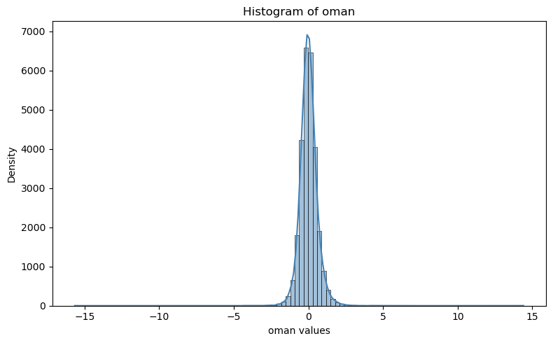
example 1#
plt.figure(figsize=(8, 5))
#sns.histplot(df["oman"], bins=50, kde=True, color="steelblue")
sns.histplot(t133.t.oman, bins=100, kde=True, color="steelblue")
plt.title("Histogram of oman")
plt.xlabel("oman values")
plt.ylabel("Density")
plt.tight_layout()
plt.show()
example 2#
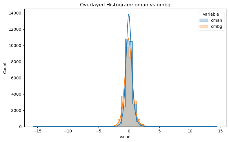
df_long = df[["oman", "ombg"]].melt(var_name="variable", value_name="value")

plt.figure(figsize=(8, 5))
sns.histplot(data=df_long, x="value", hue="variable", bins=50, kde=True, element="step", stat="count")
plt.title("Overlayed Histogram: oman vs ombg")
plt.tight_layout()
plt.show()
example 3#
plt.figure(figsize=(8, 5))
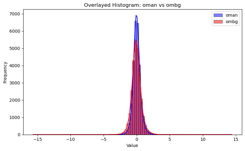
sns.histplot(df["oman"], bins=100, kde=True, color="blue", label="oman", multiple="layer")
sns.histplot(df["ombg"], bins=100, kde=True, color="red", label="ombg", multiple="layer")

plt.title("Overlayed Histogram: oman vs ombg")
plt.xlabel("Value")
plt.ylabel("Frequency")
plt.legend()
plt.tight_layout()
plt.show()
plot fitting rate#
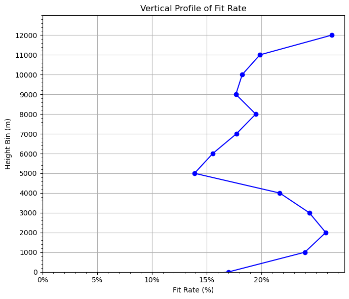
The rate fitting to observtions is an important metric to evaluate data assimilation performance.
We don’t want a small fitting rate, which means very little observation impacts on the model forecast.
We don’t want a large fitting rate either, which means we fit too close to the obervations and the model forecast will crash.
Ususally, a fitting rate of 20%~30% is expected.
# Filter valid data (both 'oman' and 'ombg' are not NaN)
valid_df = df[df["oman"].notna() & df["ombg"].notna()].copy()
valid_df = valid_df.dropna(subset=["height"])  # removes any rows in valid_df where height is missing (NaN)
# print(valid_df[valid_df["height"] < 0]["height"])   # negative height
dz = 1000
grouped = fit_rate(t133.t, dz=dz)

# 5. Plot vertical profile of fit_rate vs height
plt.figure(figsize=(7, 6))
plt.plot(grouped["fit_rate"], grouped["height_bin"], marker="o", color="blue")
# plt.axvline(x=0, color="gray", linestyle="--")  # ax vertical line

plt.xlabel("Fit Rate (%)")  # label change
plt.gca().xaxis.set_major_formatter(plt.FuncFormatter(lambda x, _: f'{x*100:.0f}%'))  # format as %
plt.ylabel("Height Bin (m)")
plt.title("Vertical Profile of Fit Rate")

# Fine-tune ticks
plt.xticks(np.arange(0, 0.25, 0.05))  #, fontsize=12)
plt.yticks(np.arange(0, 13000, dz))  #, , fontsize=12)
# Add minor ticks
from matplotlib.ticker import AutoMinorLocator
plt.gca().xaxis.set_minor_locator(AutoMinorLocator())
plt.gca().yaxis.set_minor_locator(AutoMinorLocator())
# plt.grid(which='both', linestyle='--', linewidth=0.5)
plt.grid(True)

plt.ylim(0, 13000)  # set y-axis from 0 (bottom) to 13,000 (top)
plt.tight_layout()
plt.show()
OMA: bias=0.0041 rms=0.6253
OMB: bias=-0.0494 rms=0.7753
Overall fit_rate: 19.3578%
0, -1000, 1.0682, 1.1047, 3.3063%
1, 0, 0.8419, 1.0140, 16.9675%
2, 1000, 0.6642, 0.8734, 23.9579%
3, 2000, 0.5008, 0.6755, 25.8704%
4, 3000, 0.5067, 0.6699, 24.3720%
5, 4000, 0.5604, 0.7154, 21.6729%
6, 5000, 0.7110, 0.8257, 13.8874%
7, 6000, 0.7228, 0.8560, 15.5540%
8, 7000, 0.5317, 0.6462, 17.7125%
9, 8000, 0.5192, 0.6448, 19.4768%
10, 9000, 0.5423, 0.6587, 17.6651%
11, 10000, 0.5681, 0.6949, 18.2439%
12, 11000, 0.6573, 0.8202, 19.8591%
13, 12000, 0.6994, 0.9505, 26.4228%
print(grouped["height_bin"])
0     -1000
1         0
2      1000
3      2000
4      3000
5      4000
6      5000
7      6000
8      7000
9      8000
10     9000
11    10000
12    11000
13    12000
Name: height_bin, dtype: int32
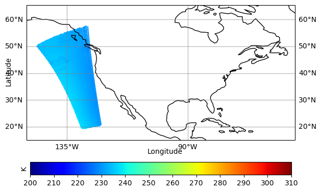
plot satellite observations#
load satellite data using obsSpace#
%%time

cris_file = f"{pyDAmonitor_ROOT}/data/mpasjedi/jdiag_cris-fsr_n20.nc"
obsCris = obsSpace(cris_file)
CPU times: user 5.67 s, sys: 2.71 s, total: 8.38 s
Wall time: 24.4 s
query_data(obsCris.bt, meta_exclude="sensorCentralWavenumber_") # removing the meta_exclude paramter will output all sensorCentralWavenumber_* information
DerivedObsError, DerivedObsValue, CloudDetectMinResidualIR, NearSSTRetCheckIR, ScanEdgeRemoval, GrossCheck, Thinning, UseflagCheck, EffectiveError0, EffectiveError1, EffectiveError2, EffectiveQC0, EffectiveQC1, EffectiveQC2, sensorZenithAngle, satelliteIdentifier, sensorScanPosition, instrumentIdentifier, longitude, latitude, sensorViewAngle, scanLineNumber, solarZenithAngle, sensorChannelNumber, sensorAzimuthAngle, fieldOfViewNumber, dateTime, solarAzimuthAngle, ObsBias0, ObsBias1, ObsBias2, constantPredictor, emissivityJacobianPredictor, hofx0, hofx1, hofx2, innov1, lapseRatePredictor, lapseRate_order_2Predictor, oman, ombg, sensorScanAnglePredictor, sensorScanAngle_order_2Predictor, sensorScanAngle_order_3Predictor, sensorScanAngle_order_4Predictor, Channel, Location
print(obsCris.bt.hofx0)
[[-- -- -- ... -- -- --]
 [222.63551330566406 224.9462127685547 222.70394897460938 ...
  291.0711669921875 291.02618408203125 290.8084411621094]
 [-- -- -- ... -- -- --]
 ...
 [-- -- -- ... -- -- --]
 [-- -- -- ... -- -- --]
 [-- -- -- ... -- -- --]]
assemble target obs array#
ncount=0
idx = []
idx2 = []
ch=61
for n in np.arange(len(obsCris.bt.ombg[:,ch])):
    #if obsCris.bt.CloudDetectMinResidualIR[n,ch] == 1:
     if obsCris.bt.ombg[n,ch] > -200 and obsCris.bt.ombg[n,ch] < 200:
       idx.append(n)
       ncount = ncount + 1

lat=obsCris.bt.latitude[idx]
lon=obsCris.bt.longitude[idx]
obarray=obsCris.bt.DerivedObsValue[idx,ch]
print(lon,lat,obarray)
print(ncount)
[-127.40092 -129.51625 -131.27661 ... -132.82477 -135.50513 -137.78625] [24.14625 24.23062 24.33297 ... 47.29415 47.29884 47.30563] [233.91612 235.93317 237.10016 ... 232.89937 233.92868 234.85745]
9521
prepare coloar map#
datmi = np.nanmin(obarray)  # Min of the data
datma = np.nanmax(obarray)  # Max of the data

if np.nanmin(obarray) < 0:
  cmax = datma
  cmin = datmi
  cmax=310
  cmin=200
  #cmax=1.0
  #cmin=-1.0
  cmap = 'RdBu'
else:
  #cmax = omean+stdev
  #cmin = np.maximum(omean-stdev, 0.0)
  cma = datma
  cmin = datmi
  cmax=310
  cmin=200
  #cmax=1.0
  #cmin=-1.0
  cmap = 'RdBu'
  cmap = 'viridis'
  cmap = 'jet'


cmin = 200.
cmax = 310.
conus_12km = [-150, -50, 15, 55]

color_map = plt.cm.get_cmap(cmap)
reversed_color_map = color_map.reversed()
units = 'K'
#units = '%'
fig = plt.figure(figsize=(10, 5))
/tmp/ipykernel_3148501/1360930195.py:30: MatplotlibDeprecationWarning: The get_cmap function was deprecated in Matplotlib 3.7 and will be removed in 3.11. Use ``matplotlib.colormaps[name]`` or ``matplotlib.colormaps.get_cmap()`` or ``pyplot.get_cmap()`` instead.
  color_map = plt.cm.get_cmap(cmap)
<Figure size 1000x500 with 0 Axes>
make the plot#
import cartopy.crs as ccrs
import matplotlib.ticker as mticker
import matplotlib.colors as colors

ax = plt.axes(projection=ccrs.PlateCarree(central_longitude=0))

# Plot grid lines
# ----------------
gl = ax.gridlines(crs=ccrs.PlateCarree(central_longitude=0), draw_labels=True,
                  linewidth=1, color='gray', alpha=0.5, linestyle='-')
gl.top_labels = False
gl.xlabel_style = {'size': 10, 'color': 'black'}
gl.ylabel_style = {'size': 10, 'color': 'black'}
gl.xlocator = mticker.FixedLocator(
   [-180, -135, -90, -45, 0, 45, 90, 135, 179.9])
ax.set_ylabel("Latitude",  fontsize=7)
ax.set_xlabel("Longitude", fontsize=7)

# Get scatter data
# ------------------
sc = ax.scatter(lon, lat,
                c=obarray, s=4, linewidth=0,
                transform=ccrs.PlateCarree(), cmap=cmap, vmin=cmin, vmax = cmax, norm=None, antialiased=True)

# Plot colorbar
# --------------
cbar = plt.colorbar(sc, ax=ax, orientation="horizontal", pad=.1, fraction=0.06,ticks=[200, 210, 220, 230, 240, 250, 260, 270, 280, 290, 300, 310])
#cbar = plt.colorbar(sc, ax=ax, orientation="horizontal", pad=.1, fraction=0.06,ticks=[-3, -2.5, -2, -1.5, -1, -0.5, 0, 0.5, 1.0, 1.5, 2.0, 2.5, 3 ])
#cbar = plt.colorbar(sc, ax=ax, orientation="horizontal", pad=.1, fraction=0.06,ticks=[0, 10, 20, 20, 40, 50, 60, 70, 80, 90, 100])
cbar.ax.set_ylabel(units, fontsize=10)
# Plot globally
# --------------
#ax.set_global()
#ax.set_extent(conus)
ax.set_extent(conus_12km)

# Draw coastlines
# ----------------
ax.coastlines()
ax.text(0.45, -0.1, 'Longitude', transform=ax.transAxes, ha='left')
ax.text(-0.08, 0.4, 'Latitude', transform=ax.transAxes,
        rotation='vertical', va='bottom')

#text = f"Total Count:{datcont:0.0f}, Max/Min/Mean/Std: {datma:0.3f}/{datmi:0.3f}/{omean:0.3f}/{stdev:0.3f} {units}"
#print(text)
#ax.text(0.67, -0.1, text, transform=ax.transAxes, va='bottom', fontsize=6.2)

dpi=100
gl.top_labels = False
plt.tight_layout()

# show plot
# -----------
# pname='test.png'
# plt.savefig(pname, dpi=dpi)