work with GSI diag files

This notebook illustreate how to work with GSI diag files using a similar obsSpaceGSI class

%%time 

# autoload external python modules if they changed
%load_ext autoreload
%autoreload 2

import os, sys
pyDAmonitor_ROOT=os.getenv("pyDAmonitor_ROOT")
if pyDAmonitor_ROOT is None:
    print("!!! pyDAmonitor_ROOT is NOT set. Run `source ush/load_pyDAmonitor.sh`")
else:
    print(f"pyDAmonitor_ROOT={pyDAmonitor_ROOT}\n")
sys.path.insert(0, pyDAmonitor_ROOT)
    
# import modules
import warnings
import math
import numpy as np
import uxarray as ux
import xarray as xr
import pandas as pd
import seaborn as sns  # seaborn handles NaN values automatically
import matplotlib.pyplot as plt
from netCDF4 import Dataset
from DAmonitor.base import query_dataset, query_data, query_obj, to_dataframe

pyDAmonitor_ROOT=/home/Guoqing.Ge/pyDAmonitor

CPU times: user 3.23 s, sys: 1.11 s, total: 4.34 s
Wall time: 5.03 s

diag_ana=f"{pyDAmonitor_ROOT}/data/gsi/diag_conv_t_anl.2024050601.nc4"
diag_bkg=f"{pyDAmonitor_ROOT}/data/gsi/diag_conv_t_ges.2024050601.nc4"

Use obsSpaceGSI to read GSI diag files

from DAmonitor.obs import obsSpaceGSI, fit_rate
tana=obsSpaceGSI(diag_ana)
tbkg=obsSpaceGSI(diag_bkg)

query_obj(tana)
# one can access diag data using `tana.data`
# query_data(tana.data)

['data', 'ds', 'filepath']

print(tana.data.Observation_Class)

['      t' '      t' '      t' ... '      t' '      t' '      t']

convert to Pandas DataFrame

pd.set_option('display.max_columns', None)  # show all dataframe columns
dfana=to_dataframe(tana.data)
dfbkg=to_dataframe(tbkg.data)
pd.set_option("display.max_columns", None)
dfana

	Station_ID	Observation_Class	Observation_Type	Observation_Subtype	Latitude	Longitude	Station_Elevation	Pressure	Height	Time	Prep_QC_Mark	Setup_QC_Mark	Prep_Use_Flag	Analysis_Use_Flag	Nonlinear_QC_Rel_Wgt	Errinv_Input	Errinv_Adjust	Errinv_Final	Observation	Obs_Minus_Forecast_adjusted	Obs_Minus_Forecast_unadjusted	Data_Pof	Data_Vertical_Velocity	Bias_Correction_1	Bias_Correction_2	Bias_Correction_3
0	AU0330	t	131	0	30.026100	236.154800	12400.0	181.500000	12400.0	-0.91944	1.0	1.0	101.0	-1.0	4.0	1.029786	1.029786	1.029786e+00	207.149994	-1.627310	-1.627310	-9.990000e+09	-9.990000e+09	-9.990000e+09	-9.990000e+09	-9.990000e+09
1	AU0330	t	131	0	30.130800	236.333405	12400.0	181.500000	12400.0	-0.89500	1.0	1.0	101.0	-1.0	4.0	1.029786	1.029786	1.029786e+00	206.949997	-1.646028	-1.646028	-9.990000e+09	-9.990000e+09	-9.990000e+09	-9.990000e+09	-9.990000e+09
2	AU0330	t	131	0	30.636900	237.190308	12400.0	181.500000	12400.0	-0.77833	1.0	1.0	101.0	-1.0	4.0	1.029786	1.029786	1.029786e+00	207.149994	-0.819473	-0.819473	-9.990000e+09	-9.990000e+09	-9.990000e+09	-9.990000e+09	-9.990000e+09
3	XZRFGAZA	t	133	0	34.238998	236.003998	10669.0	238.399994	10669.0	-0.70000	1.0	1.0	0.0	1.0	4.0	1.130850	1.130850	1.130850e+00	221.649994	-0.078072	-0.078072	-9.990000e+09	-9.990000e+09	-9.990000e+09	-9.990000e+09	-9.990000e+09
4	XZRFGAZA	t	133	0	34.234001	235.731003	10669.0	238.399994	10669.0	-0.66667	1.0	1.0	0.0	1.0	4.0	1.130850	1.130850	1.130850e+00	221.449997	-0.189546	-0.189546	-9.990000e+09	-9.990000e+09	-9.990000e+09	-9.990000e+09	-9.990000e+09
...	...	...	...	...	...	...	...	...	...	...	...	...	...	...	...	...	...	...	...	...	...	...	...	...	...	...
63560	F4586	t	188	0	46.589169	298.989838	47.0	1018.400024	47.0	0.00000	2.0	1.0	101.0	-1.0	4.0	0.250000	0.250000	1.000000e-10	282.049988	2.429230	2.446748	-9.990000e+09	-9.990000e+09	-9.990000e+09	-9.990000e+09	-9.990000e+09
63561	F9448	t	188	0	46.615002	298.967621	19.0	1021.500000	19.0	0.00000	2.0	1.0	101.0	-1.0	4.0	0.250000	0.250000	1.000000e-10	278.750000	0.310210	-1.171543	-9.990000e+09	-9.990000e+09	-9.990000e+09	-9.990000e+09	-9.990000e+09
63562	F3942	t	188	0	46.642830	298.998322	11.0	1022.700012	11.0	0.00000	2.0	1.0	101.0	-1.0	4.0	0.250000	0.250000	1.000000e-10	280.950012	1.367755	0.994733	-9.990000e+09	-9.990000e+09	-9.990000e+09	-9.990000e+09	-9.990000e+09
63563	G0274	t	188	0	46.645828	299.047485	10.0	1022.700012	10.0	0.00000	2.0	1.0	101.0	-1.0	4.0	0.250000	0.250000	1.000000e-10	282.049988	2.479401	2.336636	-9.990000e+09	-9.990000e+09	-9.990000e+09	-9.990000e+09	-9.990000e+09
63564	F2780	t	188	0	46.824669	299.187317	42.0	1019.000000	42.0	0.00000	2.0	1.0	101.0	-1.0	4.0	0.250000	0.250000	1.000000e-10	280.950012	2.195708	0.297975	-9.990000e+09	-9.990000e+09	-9.990000e+09	-9.990000e+09	-9.990000e+09

63565 rows × 26 columns

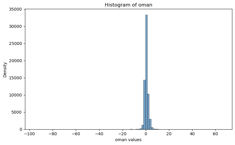
Plot histrogram

plt.figure(figsize=(8, 5))
#sns.histplot(df["oman"], bins=50, kde=True, color="steelblue")
sns.histplot(tana.data.Obs_Minus_Forecast_adjusted, bins=100, kde=False, color="steelblue")
plt.title("Histogram of oman")
plt.xlabel("oman values")
plt.ylabel("Density")
plt.tight_layout()
plt.show()

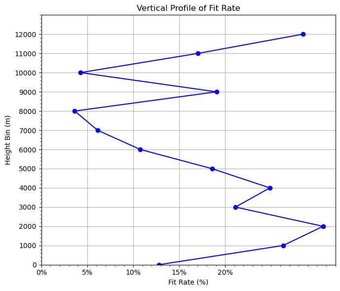
Plot fitting rate

## assemble 133 OMB and OMA into a dictionary
df_133_a = dfana[dfana["Observation_Type"] == 133]
df_133_b = dfbkg[dfbkg["Observation_Type"] == 133]

t133={
    'oman': df_133_a["Obs_Minus_Forecast_adjusted"].to_numpy(),
    'ombg': df_133_b["Obs_Minus_Forecast_adjusted"].to_numpy(),
    'height': df_133_a["Station_Elevation"].to_numpy(),
}

dz = 1000
grouped = fit_rate(t133, dz=dz)

# 5. Plot vertical profile of fit_rate vs height
plt.figure(figsize=(7, 6))
plt.plot(grouped["fit_rate"], grouped["height_bin"], marker="o", color="blue")
# plt.axvline(x=0, color="gray", linestyle="--")  # ax vertical line

plt.xlabel("Fit Rate (%)")  # label change
plt.gca().xaxis.set_major_formatter(plt.FuncFormatter(lambda x, _: f'{x*100:.0f}%'))  # format as %
plt.ylabel("Height Bin (m)")
plt.title("Vertical Profile of Fit Rate")

# Fine-tune ticks
plt.xticks(np.arange(0, 0.25, 0.05))  #, fontsize=12)
plt.yticks(np.arange(0, 13000, dz))  #, , fontsize=12)
# Add minor ticks
from matplotlib.ticker import AutoMinorLocator
plt.gca().xaxis.set_minor_locator(AutoMinorLocator())
plt.gca().yaxis.set_minor_locator(AutoMinorLocator())
# plt.grid(which='both', linestyle='--', linewidth=0.5)
plt.grid(True)

plt.ylim(0, 13000)  # set y-axis from 0 (bottom) to 13,000 (top)
plt.tight_layout()
plt.show()

OMA: bias=0.0242 rms=1.2549
OMB: bias=0.2107 rms=1.4361
Overall fit_rate: 12.6145%
0, -1000, 1.2516, 1.7449, 28.2731%
1, 0, 1.6060, 1.8412, 12.7736%
2, 1000, 0.8703, 1.1811, 26.3083%
3, 2000, 0.7375, 1.0638, 30.6658%
4, 3000, 0.7399, 0.9380, 21.1196%
5, 4000, 0.7347, 0.9778, 24.8696%
6, 5000, 1.2334, 1.5148, 18.5773%
7, 6000, 1.4749, 1.6529, 10.7703%
8, 7000, 1.7494, 1.8635, 6.1250%
9, 8000, 1.5833, 1.6431, 3.6373%
10, 9000, 0.6370, 0.7869, 19.0587%
11, 10000, 1.7016, 1.7773, 4.2578%
12, 11000, 0.7794, 0.9396, 17.0520%
13, 12000, 1.0761, 1.5041, 28.4568%

For reference, check diag file contents using netCDF4 directly

dataset=Dataset(diag_ana, mode='r')
query_dataset(dataset)

Station_ID, Observation_Class, Observation_Type, Observation_Subtype, Latitude, Longitude, Station_Elevation, Pressure, Height, Time, Prep_QC_Mark, Setup_QC_Mark, Prep_Use_Flag, Analysis_Use_Flag, Nonlinear_QC_Rel_Wgt, Errinv_Input, Errinv_Adjust, Errinv_Final, Observation, Obs_Minus_Forecast_adjusted, Obs_Minus_Forecast_unadjusted, Data_Pof, Data_Vertical_Velocity, Bias_Correction_Terms

check the shape/ndim of each variable in the netCDF4 dataset

for var in dataset.variables:
    print(var, dataset.variables[var][:].shape) #ndim

Station_ID (63565, 8)
Observation_Class (63565, 7)
Observation_Type (63565,)
Observation_Subtype (63565,)
Latitude (63565,)
Longitude (63565,)
Station_Elevation (63565,)
Pressure (63565,)
Height (63565,)
Time (63565,)
Prep_QC_Mark (63565,)
Setup_QC_Mark (63565,)
Prep_Use_Flag (63565,)
Analysis_Use_Flag (63565,)
Nonlinear_QC_Rel_Wgt (63565,)
Errinv_Input (63565,)
Errinv_Adjust (63565,)
Errinv_Final (63565,)
Observation (63565,)
Obs_Minus_Forecast_adjusted (63565,)
Obs_Minus_Forecast_unadjusted (63565,)
Data_Pof (63565,)
Data_Vertical_Velocity (63565,)
Bias_Correction_Terms (63565, 3)

print(dataset.variables["Bias_Correction_Terms"][:])

[[-9.99e+09 -9.99e+09 -9.99e+09]
 [-9.99e+09 -9.99e+09 -9.99e+09]
 [-9.99e+09 -9.99e+09 -9.99e+09]
 ...
 [-9.99e+09 -9.99e+09 -9.99e+09]
 [-9.99e+09 -9.99e+09 -9.99e+09]
 [-9.99e+09 -9.99e+09 -9.99e+09]]

check attributes

for stmp in dataset.variables["Data_Pof"].ncattrs():
    print(stmp)

print(dataset.variables["Data_Pof"].ncattrs())

[]