Find and plot individual MPAS cells#
Find cell index based on terrain plots in a map
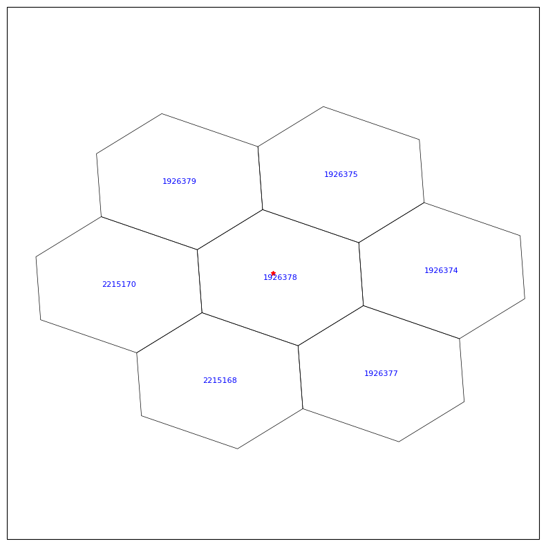
Find all neighborhood cells based on an input lat/lon
etc
get the pyDAmonitor_ROOT env variable#
This step is highly recommended. It is required if one want to use the DAmonitor Python package or use the MPAS/FV3 sample data or local cartopy nature_earth_data.
%%time
# autoload external python modules if they changed
%load_ext autoreload
%autoreload 2
import sys, os
pyDAmonitor_ROOT=os.getenv("pyDAmonitor_ROOT")
if pyDAmonitor_ROOT is None:
print("!!! pyDAmonitor_ROOT is NOT set. Run `source ush/load_pyDAmonitor.sh`")
else:
print(f"pyDAmonitor_ROOT={pyDAmonitor_ROOT}\n")
sys.path.insert(0, pyDAmonitor_ROOT)
pyDAmonitor_ROOT=/ncrc/home2/Guoqing.Ge/pyDAmonitor
CPU times: user 7.73 ms, sys: 29.7 ms, total: 37.4 ms
Wall time: 168 ms
import modules#
%%time
import numpy as np
from netCDF4 import Dataset
import matplotlib.pyplot as plt
import matplotlib as mpl
import cartopy
import cartopy.crs as ccrs
import cartopy.feature as cfeature
from DAmonitor.base import query_dataset, query_obj
cartopy.config['data_dir'] = f"{pyDAmonitor_ROOT}/data/natural_earth_data"
CPU times: user 7.46 s, sys: 165 ms, total: 7.63 s
Wall time: 1.37 s
read in invariant.nc#
ds0 = Dataset(os.path.join(pyDAmonitor_ROOT,'data/mpasjedi/invariant.nc'), 'r')
query_dataset(ds0)
xtime, Time, latCell, lonCell, xCell, yCell, zCell, indexToCellID, latEdge, lonEdge, xEdge, yEdge, zEdge, indexToEdgeID, latVertex, lonVertex, xVertex, yVertex, zVertex, indexToVertexID, cellsOnEdge, nEdgesOnCell, nEdgesOnEdge, edgesOnCell, edgesOnEdge, weightsOnEdge, dvEdge, dcEdge, angleEdge, areaCell, areaTriangle, cellsOnCell, verticesOnCell, verticesOnEdge, edgesOnVertex, cellsOnVertex, kiteAreasOnVertex, meshDensity, nominalMinDc, bdyMaskCell, bdyMaskEdge, bdyMaskVertex, edgeNormalVectors, localVerticalUnitVectors, cellTangentPlane, fEdge, fVertex, ter, landmask, mminlu, isice_lu, iswater_lu, ivgtyp, landusef, soilf, isltyp, snoalb, soiltemp, greenfrac, shdmin, shdmax, albedo12m, lai12m, soilcomp, soilcl1, soilcl2, soilcl3, soilcl4, var2d, con, oa1, oa2, oa3, oa4, ol1, ol2, ol3, ol4, deriv_two, defc_a, defc_b, cell_gradient_coef_x, cell_gradient_coef_y, coeffs_reconstruct, cf1, cf2, cf3, zgrid, rdzw, dzu, rdzu, fzm, fzp, zxu, zz, zb, zb3, dss
check indexToCellID, attributes, dimensions, etc#
print(ds0["indexToCellID"][:])
# print(ds0.ncattrs())
print(ds0.dimensions.keys())
print(ds0.dimensions["nVertLevels"].size)
print(ds0.dimensions["nCells"].size)
ds0.dimensions
# ds0
[ 1 2 3 ... 2341816 2341817 2341818]
dict_keys(['StrLen', 'Time', 'nCells', 'nEdges', 'nVertices', 'TWO', 'maxEdges', 'maxEdges2', 'vertexDegree', 'R3', 'nlcat', 'nscat', 'nMonths', 'nSoilComps', 'FIFTEEN', 'nVertLevelsP1', 'nVertLevels'])
59
2341818
{'StrLen': "<class 'netCDF4.Dimension'>": name = 'StrLen', size = 64,
'Time': "<class 'netCDF4.Dimension'>" (unlimited): name = 'Time', size = 1,
'nCells': "<class 'netCDF4.Dimension'>": name = 'nCells', size = 2341818,
'nEdges': "<class 'netCDF4.Dimension'>": name = 'nEdges', size = 7031657,
'nVertices': "<class 'netCDF4.Dimension'>": name = 'nVertices', size = 4689840,
'TWO': "<class 'netCDF4.Dimension'>": name = 'TWO', size = 2,
'maxEdges': "<class 'netCDF4.Dimension'>": name = 'maxEdges', size = 6,
'maxEdges2': "<class 'netCDF4.Dimension'>": name = 'maxEdges2', size = 12,
'vertexDegree': "<class 'netCDF4.Dimension'>": name = 'vertexDegree', size = 3,
'R3': "<class 'netCDF4.Dimension'>": name = 'R3', size = 3,
'nlcat': "<class 'netCDF4.Dimension'>": name = 'nlcat', size = 20,
'nscat': "<class 'netCDF4.Dimension'>": name = 'nscat', size = 16,
'nMonths': "<class 'netCDF4.Dimension'>": name = 'nMonths', size = 12,
'nSoilComps': "<class 'netCDF4.Dimension'>": name = 'nSoilComps', size = 8,
'FIFTEEN': "<class 'netCDF4.Dimension'>": name = 'FIFTEEN', size = 15,
'nVertLevelsP1': "<class 'netCDF4.Dimension'>": name = 'nVertLevelsP1', size = 60,
'nVertLevels': "<class 'netCDF4.Dimension'>": name = 'nVertLevels', size = 59}
check zgrid, ter#
print(ds0["zgrid"].shape)
print(ds0["zgrid"][2341817,:])
print(ds0["zgrid"][50,:])
print(ds0["ter"][2341817])
print(ds0["ter"][50])
ds0["zgrid"]
(2341818, 60)
[ 167.82333 185.77321 206.06612 229.00009 254.90726 284.15988
317.1729 354.40787 396.37677 443.64685 496.84344 556.6553
623.838 699.2172 783.6908 878.2324 983.8933 1101.8014
1233.1609 1379.2413 1541.3639 1720.8761 1919.1221 2137.4119
2376.9902 2639.0088 2924.4958 3234.3262 3569.1953 3929.5994
4315.8257 4727.9414 5165.782 5628.9395 6116.748 6628.2944
7162.4326 7717.8213 8292.971 8886.258 9495.987 10120.584
10758.49 11410.003 12083.912 12781.494 13502.739 14247.813
15017.097 15811.2295 16631.184 17478.498 18355.48 19265.338
20212.562 21206.213 22256.027 23373.223 24573.371 25878.713 ]
[ 1019.22375 1037.1692 1057.4492 1080.3549 1106.2078 1135.3682
1168.2329 1205.242 1246.8772 1293.6632 1346.1683 1405.0109
1470.8481 1544.3793 1626.3389 1717.4945 1818.6484 1930.6416
2054.3857 2190.8994 2341.3638 2507.1667 2689.8967 2891.2744
3113.0166 3356.6953 3623.6172 3914.7493 4230.679 4571.6016
4937.346 5327.4453 5741.2305 6177.9424 6636.809 7117.082
7617.9907 8138.6885 8678.219 9235.593 9809.8125 10399.661
11003.978 11623.366 12266.561 12935.18 13629.592 14350.281
15097.869 15873.15 16677.15 17511.363 18377.943 19279.871
20221.344 21211.059 22258.389 23374.19 24573.674 25878.713 ]
167.82333
1019.22375
<class 'netCDF4.Variable'>
float32 zgrid(nCells, nVertLevelsP1)
units: m MSL
long_name: Geometric height of layer interfaces
unlimited dimensions:
current shape = (2341818, 60)
filling on, default _FillValue of 9.969209968386869e+36 used
compute a new zgrid by removing the terrain height#
%%time
agl=np.empty_like(ds0["zgrid"][:])
for i in range(60):
agl[:,i]=ds0["zgrid"][:,i]-ds0["ter"][:]
CPU times: user 3.62 s, sys: 27.3 s, total: 30.9 s
Wall time: 31.1 s
np.set_printoptions(suppress=True) # disables scientific notation
np.set_printoptions(precision=3) # optional: 2 decimal places
print(agl[2341817,:])
print(agl[50,:]) # the AGL zgrid values are different at different locations
[ 0. 17.95 38.243 61.177 87.084 116.337 149.35
186.585 228.553 275.824 329.02 388.832 456.015 531.394
615.867 710.409 816.07 933.978 1065.338 1211.418 1373.541
1553.053 1751.299 1969.589 2209.167 2471.186 2756.673 3066.503
3401.372 3761.776 4148.002 4560.118 4997.959 5461.116 5948.925
6460.471 6994.609 7549.998 8125.147 8718.435 9328.164 9952.761
10590.667 11242.18 11916.089 12613.671 13334.916 14079.99 14849.273
15643.406 16463.36 17310.674 18187.656 19097.514 20044.738 21038.389
22088.203 23205.398 24405.547 25710.889]
[ 0. 17.945 38.225 61.131 86.984 116.144 149.009
186.018 227.653 274.439 326.945 385.787 451.624 525.156
607.115 698.271 799.425 911.418 1035.162 1171.676 1322.14
1487.943 1670.673 1872.051 2093.793 2337.472 2604.394 2895.525
3211.456 3552.378 3918.123 4308.222 4722.007 5158.719 5617.585
6097.858 6598.767 7119.465 7658.995 8216.369 8790.589 9380.438
9984.754 10604.143 11247.337 11915.956 12610.368 13331.058 14078.646
14853.927 15657.927 16492.139 17358.719 18260.646 19202.12 20191.834
21239.164 22354.965 23554.45 24859.488]
scatter-plot all cell terrain values and when a mouse hovers on a cell, show its lat,lon,ter and iCell (cell index)#
Write down the target cell index and then we can print a field profile for that cell
import plotly.express as px
import xarray as xr
import plotly.io as pio
pio.renderers.default = 'notebook'
# plot the whole map
factor=50 # plotting all cells take too many memories, so plot every factor cells
lon = np.degrees(ds0.variables['lonCell'][::factor])
lat = np.degrees(ds0.variables['latCell'][::factor])
iCell = ds0.variables['indexToCellID'][::factor]
ter = ds0["ter"][::factor]
# plot a subdomain defined by latmin, latmax, lonmin, lonmax
# latmin, latmax = 37, 41
# lonmin0, lonmax0 = -109, -102
# #
# lon0 = np.degrees(ds0.variables['lonCell'][:])
# lat0 = np.degrees(ds0.variables['latCell'][:])
# lonmin = lonmin0 + 360
# lonmax = lonmax0 + 360
# mask = (lat0 >= latmin) & (lat0 <= latmax) & (lon0 >= lonmin) & (lon0 <= lonmax)
# lat = lat0[mask]
# lon = lon0[mask]
# iCell = ds0.variables['indexToCellID'][:][mask]
# ter = ds0.variables["ter"][:][mask]
# use projections, but LLC is not natively supported in plotly
# fig = px.scatter_geo(
# lat=lat,
# lon=lon,
# color=ter,
# color_continuous_scale="Viridis", # choose any supported colorscale
# projection="mercator",
# hover_name=None, # optional: show info on hover
# hover_data={"lat": lat, "lon": lon, "ter": ter},
# size_max=10,
# )
# use maps
fig = px.scatter_map(
lat=lat,
lon=lon,
color=ter,
color_continuous_scale="Viridis", # choose any supported colorscale
hover_name=None, # optional: show info on hover
hover_data={"lat": lat, "lon": lon, "ter": ter, "iCell": iCell},
size_max=1,
)
# set width and height
fig.update_layout(
width=1000, # pixels
height=800, # pixels
title=""
)
# Show interactive map
fig.show()
Print pressure profile in the Atlantic at iCell=1702401#
iCell = 1702401
ds1 = Dataset(os.path.join(pyDAmonitor_ROOT,'data/mpasjedi/bkg.nc'), 'r')
query_dataset(ds1)
pfull = ds1['pressure_p'][:] + ds1['pressure_base'][:]
print(pfull.shape)
print(pfull[0,iCell,:])
qv, qc, qr, qi, qs, qg, ni, nr, ng, nc, nifa, nwfa, volg, initial_time, xtime, u, w, rho, pressure_p, pressure_base, theta, relhum, rho_base, theta_base, uReconstructZonal, uReconstructMeridional, surface_pressure, isltyp, soilf, ivgtyp, landusef, mminlu, isice_lu, iswater_lu, landmask, shdmin, shdmax, snoalb, albedo12m, greenfrac, lai12m, cldfrac, re_cloud, re_ice, re_snow, refl10cm_max, rainnc, lai, sfc_albbck, sfc_albedo, sfc_emibck, mavail, sfc_emiss, thc, ust, xicem, z0, znt, skintemp, snow, snowc, snowh, sst, tmn, vegfra, seaice, xice, xland, u10, v10, q2, t2m, precipw, dzs, zs, ter, sh2o, smois, tslb, h_oml_initial
(1, 2341818, 59)
[101050.21 100827.36 100575.7 100291.87 99971.98 99611.586
99206.03 98750.02 98237.805 97663.21 97019.45 96299.28
95494.914 94598.32 93601.086 92494.75 91270.93 89921.26
88437.9 86814.08 85046.22 83133.59 81072.44 78859.78
76499.64 74004.44 71381.86 68635.82 65771.73 62792.363
59712.547 56557.555 53354.227 50127.465 46902.875 43700.73
40543.67 37458.305 34464.246 31579.037 28818.988 26200.248
23719.398 21368.52 19168.184 17131.22 15242.44 13492.477
11880.851 10394.819 9037.443 7826.539 6744.678 5781.303
4931.021 4178.032 3509.6 2917.626 2393.344]
Find the top interface level pressure#
from math import log, exp
size = pfull[0,iCell,:].size
logIm1 = ( log(pfull[0,iCell,size-1]) + log(pfull[0,iCell,size-2]) ) /2
logM = log(pfull[0,iCell,size-1])
logI = 2 * logM - logIm1
exp(logI)
2167.667709920563
Find and plot neighborhood cells around a given lat, lon#
import numpy as np
import matplotlib.pyplot as plt
import cartopy.crs as ccrs
from netCDF4 import Dataset
cartopy.config['data_dir'] = f"{pyDAmonitor_ROOT}/data/natural_earth_data"
mylat, mylon0 = 40.14, -105.18 # specify a given lot, lon
lat_incr = 0.01 # degreee, ~1km?
lon_incr = 0.01 # degree, ~1km?
mylon = mylon0 + 360 # convert to 360-based degree
lonCell = np.degrees(ds0.variables['lonCell'][:])
latCell = np.degrees(ds0.variables['latCell'][:])
lonVertex = np.degrees(ds0.variables['lonVertex'][:])
latVertex = np.degrees(ds0.variables['latVertex'][:])
# Connectivity: vertices of each cell
verticesOnCell = ds0.variables['verticesOnCell'][:] # shape (nCells, maxEdges)
nEdgesOnCell = ds0.variables['nEdgesOnCell'][:]
# find neighborhood cells (>=7)
for iter in range(10):
latmin = mylat - lat_incr * (iter + 1)
latmax = mylat + lat_incr * (iter + 1)
lonmin = mylon - lon_incr * (iter + 1)
lonmax = mylon + lon_incr * (iter + 1)
maskC = (latCell >= latmin) & (latCell <= latmax) & (lonCell >= lonmin) & (lonCell <= lonmax)
latC = latCell[maskC]
lonC = lonCell[maskC]
vertC = verticesOnCell[maskC]
nEdgesC = nEdgesOnCell[maskC]
print(latC.size)
if latC.size >= 7:
break # exit the loop if we find 7+ cells
# find the cell indices
iCell = ds0.variables['indexToCellID'][:][maskC]
# ter = ds0.variables["ter"][:][mask]
# --- Plot ---
fig = plt.figure(figsize=(10, 10))
ax = plt.axes(projection=ccrs.PlateCarree())
# add costlines, country borders, state/province borders
ax.coastlines(resolution='50m') # '110m', '50m', or '10m'
ax.add_feature(cfeature.BORDERS, linewidth=0.7)
ax.add_feature(cfeature.STATES, linewidth=0.5, edgecolor='gray')
#ax.add_feature(cfeature.LAND, facecolor=cfeature.COLORS['land'])
#ax.add_feature(cfeature.OCEAN, facecolor=cfeature.COLORS['water'])
# relax the plotting extent by the "buffer" degree
buffer = 0.02
ax.set_extent([lonmin - buffer, lonmax + buffer, latmin - buffer, latmax + buffer])
# plot ploygons
for i in range(latC.size):
nEdges = nEdgesC[i]
verts = vertC[i, :nEdges] - 1 # convert 1-based to 0-based index
poly_lon = lonVertex[verts]
poly_lat = latVertex[verts]
ax.fill(poly_lon, poly_lat, edgecolor="black", facecolor="none", linewidth=0.5, transform=ccrs.PlateCarree())
# add the cell index in the center of the cell
ax.text(lonC[i], latC[i], f'{iCell[i]}',
transform=ccrs.PlateCarree(),
fontsize=8, color="blue",
ha="center", va="center")
# Plot a star at the user specificed (mylon, mylat)
ax.plot(mylon, mylat, marker="*", color="red", markersize=5, # o, ^, s
transform=ccrs.PlateCarree())
plt.show()
1
1
5
7